Calculating the inverse kinematics for a Peg Solitaire-playing delta-robot

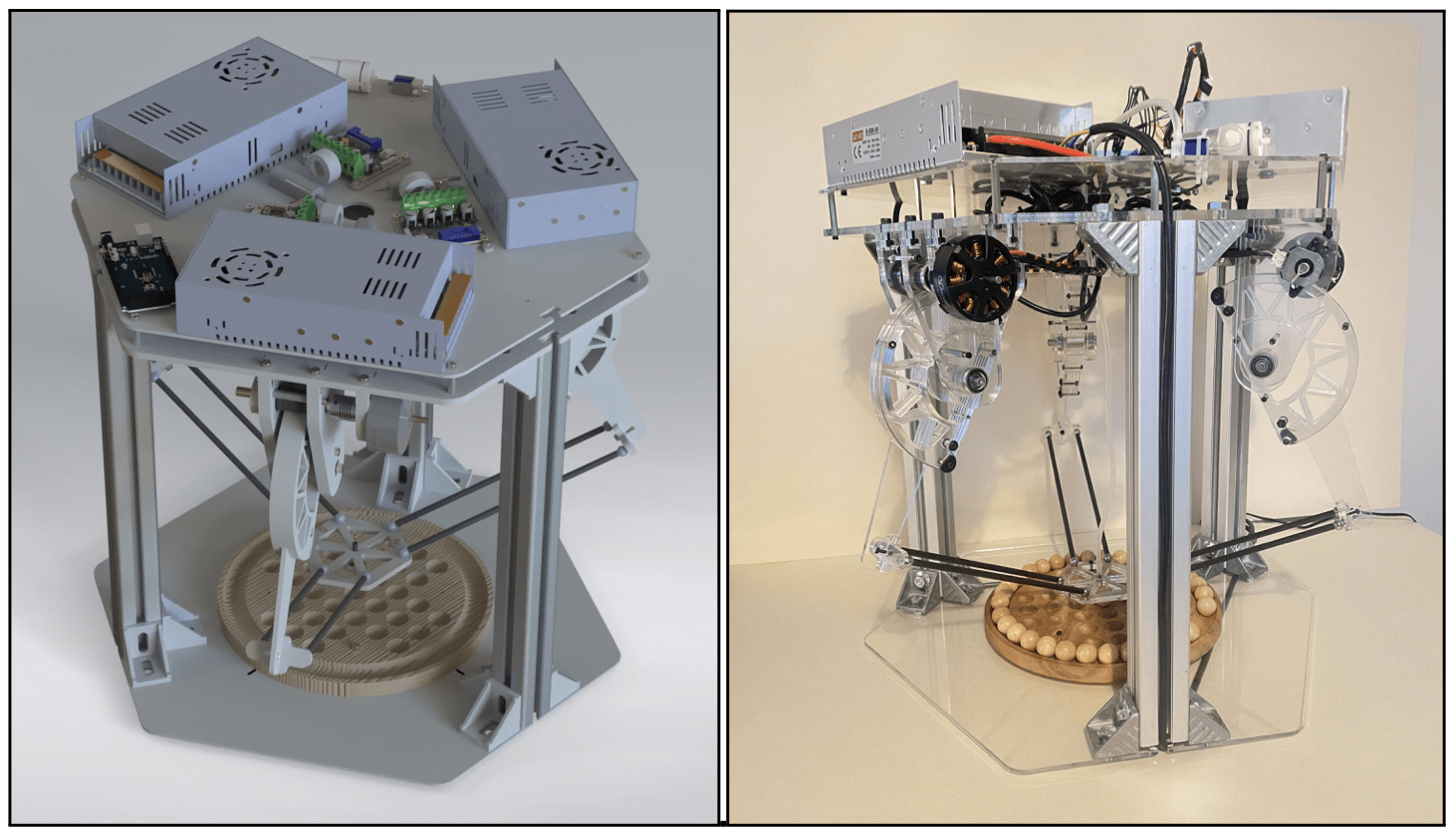
Welcome to a somewhat unorthodox post about a project that I've been working on: A Peg Solitaire-playing delta-robot. This is a hobby-project that I've been tinkering with in my spare time for a while now, and I've finally gotten the robot to work, so without further ado, let me introduce Peggy:
See Peggy win a game of Peg Solitaire in under 3 minutes
I'm a programmer by heart and love card games, which is why I created Online Solitaire and recently bought World of Card Games, but I also love tinkering with physical things, such as robots. I've designed, built, and programmed this robot from scratch, and it's without a doubt my biggest project to date. There's still a lot of potential for optimizations on the robot, but it works!
I expect this to be the first part in a series of posts where I'll go through a lot of details concerning the robot. I've put a lot of man-hours into the robot, so I hope that people who have an interest in tinkering with robots will benefit from my experiences building one.
So without further ado, let's begin at the beginning, which when creating a robot is all about the kinematic calculations. There are two types of kinematic calculations: forward kinematics and inverse kinematic. They each solve their own problem and have their own use case. This post will focus on the inverse kinematics.
The formula derived from the forward kinematic calculations can give the mobile base's position based on the actuators' angle. The mobile base is often referred to as the end effector as well, and it's where the grabbing mechanism is attached, which in this case is a suction cup. The forward kinematics can be used if corrections need to be made to the mobile base's position. For example, if a camera is used to determine the mobile base's real-life position, and it does not match the position from the kinematic calculations, the discrepancy can be determined, and corrections can be made in the robot's position.
The formula derived from the inverse kinematic calculations can give the angle of the actuators based on a given position in the x-y-z space. These calculations will form the basis for programming the movement of the robot.
Below, we'll go through the calculations for the inverse kinematics. Before we can do that, some definitions must be set for the lengths and angles that will be used in the calculations. These definitions can be seen in figure 1 below.
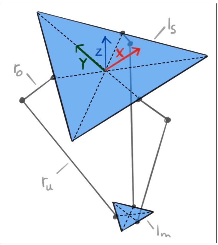
In figure 1, the stationary base and the mobile base are depicted as two equilateral triangles, both horizontal. Throughout the calculations, the length of the side of the stationary base (l_S), mobile base (l_M), and the length of the upper arm (r_O) and lower arm (r_U) will be used. The origin for the entire system is defined to be in the middle of the stationary base.
In figure 2, it can be seen that not all arms operate in the same plane, but that the lower arm can be offset from the plane that its corresponding upper arm is part of. This is because not all joints are of the same type. The stationary joint at the actuator (S1) is a rotational joint that operates in the y-z plane, where it can (theoretically) rotate in a circle with the origin in S1 and a radius of r_O. The elbow joint (A1), on the other hand, is a universal joint, and so is the joint on the mobile base (M1).
This means that r_U does not necessarily stick to a path in the y-z plane. Since both joints are universal joints and can therefore rotate freely, they can (theoretically) create a sphere with a center in M1 and a radius of r_U. The intersection between this sphere and the y-z plane is indicated by M′1, which serves as the origin in a circle with a radius of r′U. Finally, the mobile base's origin is defined as M0 and the angle between the y-axis and r_U is defined as θ1.
With all these definitions, it is now possible, using algebra, to find the point A1 as the intersection of two circles.
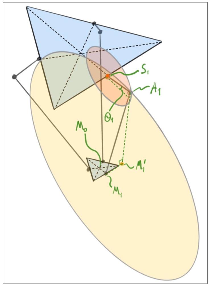
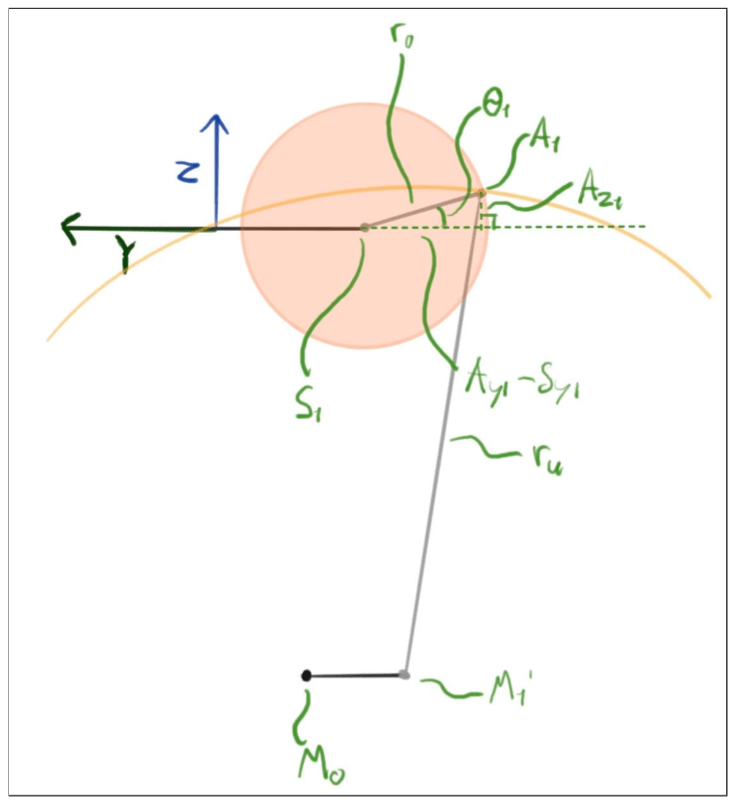
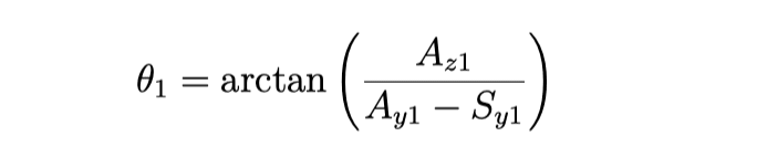
An illustration of the y-z plane can be seen in figure 3 below. A1 is the intersection point between the two aforementioned circles, so if point A1 is known, θ1 can be calculated.
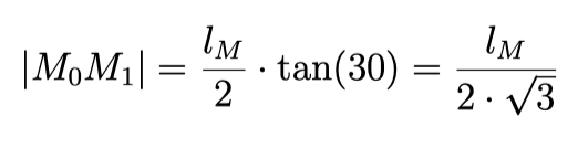
The distance between points M0 and M1 can now be found using Pythagoras. In figure 4, an illustration of the mobile base's x-y plane is seen.
The distance M0M1 is be found to be:
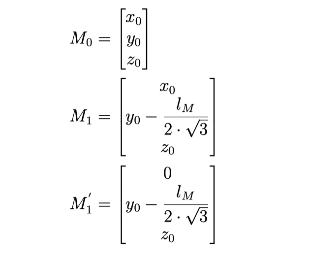
The coordinate set for the points of the mobile base can now be found:
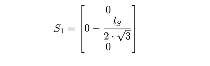
And the coordinate set for the points of the stationary base can be found:
The length from point M′1 to A1 can be calculated:

Pythagorean theorem for right-angled triangles (a2+b2=c2) can now be used for the two triangles formed by the upper and lower arms:
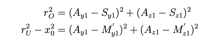
And if the known values are inserted:
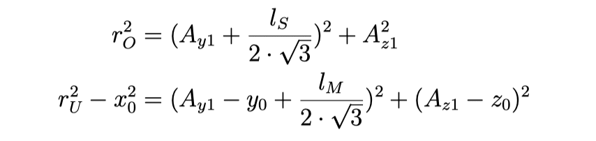
In the above two equations, only Ay1 and Az1 are unknown. We now have two equations with two unknowns, so a solution can be found. If solved symbolically, the solution looks very complex. However, all values are known, so in practice, it is not that complex. Based on the found variables, the coordinate set for A1 can be defined as:

It is now possible to find the angle θ1 by using the inverse of the trigonometric functions:
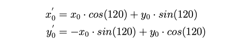
The above calculations can be reused to find θ2 and θ3. Since the robot is symmetrical, the x-y plane is simply rotated around the z-axis. This is done by defining a new x0 and y0, which are used in the calculations instead.
When this is done in the clockwise direction, the values for θ2 can be defined as:
The values for θ3 can be defined as:

Now, by inserting the actual values for the robot, the mobile base can be moved to a specific location in the x-y-z space by giving it a coordinate.